Wave solvers I: pseudo-spectral (JAXiON)

Fuzzy dark matter is simulated by evolving the wavefunction directly. The pseudo-spectral split-step method — the approach behind our JAXiON code — is unitary, spectrally accurate, and naturally differentiable. This article explains how it works.

Split-step Fourier evolution

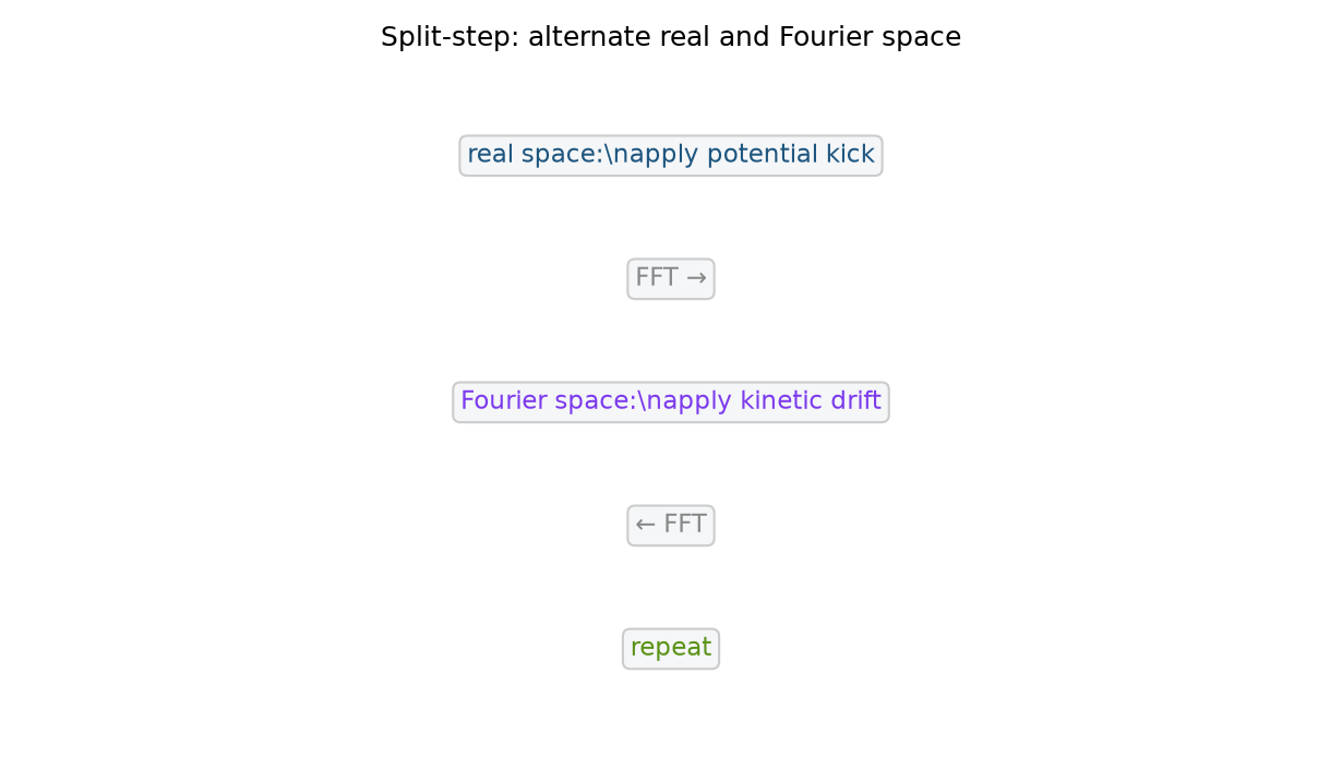
The Schrödinger equation has a kinetic part (a Laplacian, diagonal in Fourier space) and a potential part (a multiplication, diagonal in real space). The split-step method alternates: apply the potential kick in real space, FFT to Fourier space, apply the kinetic drift, FFT back. Each sub-step is exact for its operator, and the scheme is second-order accurate in the timestep.

Unitary and conservative

Because each operator is applied as a pure phase rotation, the evolution is unitary — it conserves the total mass $\int|\psi|^2$ to machine precision and is unconditionally stable. Spectral gradients (via FFT) are exact, so there is no finite-difference dispersion error. This is why spectral solvers are the reference for FDM.

Worked example — JAXiON's conservation

Our JAXiON solver conserves mass to $|\Delta M/M|\sim10^{-13}$ (machine precision, from unitarity) and energy to $\sim10^{-9}$ over 300+ checkpoints. Those numbers are the trust test: a core density or radius from a run that drifted would be meaningless. Spectral unitarity is what makes them so tight.

A wave (spectral) solver evolves $\psi$ directly, capturing the interference and cores that distinguish FDM (right) from $\Lambda$CDM (left) from identical initial conditions.

The differentiable advantage

JAXiON is written in JAX, so the entire split-step evolution is automatically differentiable: one can compute the gradient of any output (a core mass, a power spectrum) with respect to inputs like the boson mass. This turns the simulator into a differentiable model, enabling gradient-based inference (Topic 9.6) — a genuine novelty of the campaign.

The cost

The price of spectral accuracy is a uniform grid: resolution is fixed everywhere, set by the finest scale needed anywhere. For a cosmological box that must resolve the de Broglie wavelength, this is the resolution wall (Topic 9.5), and it is why spectral solvers are paired with, or give way to, adaptive-mesh methods (Topic 9.4).

The split-step cycle: alternate a real-space potential kick and a Fourier-space kinetic drift.

In our research

JAXiON is our differentiable spectral lane. Its machine-precision conservation ($|\Delta M/M|\sim10^{-13}$) validates every core it measures; its differentiability enables our boson-mass inference (Topic 9.6); and its soliton solver reproduces the Schive profile to $<1\%$ (JXE-F5) — the foundation of the core–halo result.

Key references

Mocz et al. (2017), MNRAS 471, 4559 (arXiv:1705.05845).
Edwards et al. (2018), PyUltraLight, JCAP 10, 027 (arXiv:1807.04037).
May & Springel (2021), Structure formation in FDM, MNRAS 506, 2603 (arXiv:2101.01828).

PreviousInitial conditions: from P(k) to particles NextWave solvers II: adaptive mesh (GAMER/ELBDM)