Two-point statistics: the correlation function & power spectrum

You cannot predict where each galaxy sits, only the statistics of the field. The correlation function and its Fourier partner, the power spectrum $P(k)$, capture clumpiness scale by scale — and $P(k)$ is the single input from which the transfer function, $\sigma(M)$, and the halo mass function are all built.

Measuring clumpiness

The simplest statistic of a random density field is the two-point correlation function — the excess probability, over random, of finding matter at two points separated by $r$:

$$\xi(r)=\langle\delta(\mathbf x)\,\delta(\mathbf x+\mathbf r)\rangle.$$

A positive $\xi$ at small $r$ means matter clusters; $\xi\to0$ at large $r$ means uniformity on big scales.

The power spectrum

In Fourier space the same information is the power spectrum, the variance carried by modes of wavenumber $k$:

$$\langle\delta_{\mathbf k}\,\delta^{*}_{\mathbf k'}\rangle=(2\pi)^3P(k)\,\delta_D(\mathbf k-\mathbf k'),$$

and $P(k)$ is just the Fourier transform of $\xi(r)$. For a Gaussian field — as the early Universe is, to great precision — $P(k)$ holds all the statistical information.

Reading P(k)

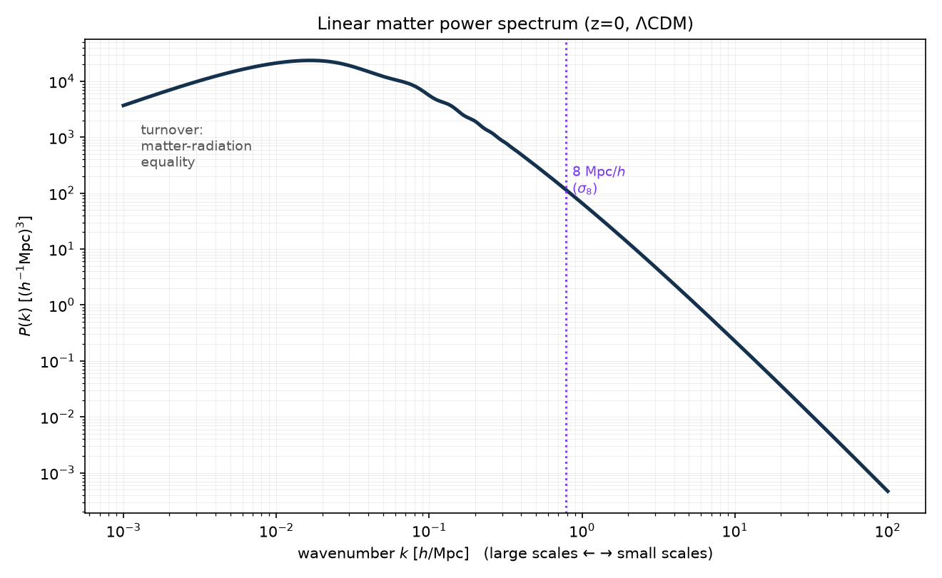
The linear $P(k)$ (figure) rises on large scales, turns over near the scale of matter–radiation equality, and falls on small scales. Large $k$ = small scales — and the small-scale end is exactly where the dark-matter model leaves its fingerprint: cold dark matter preserves power there, fuzzy dark matter cuts it off.

The linear matter power spectrum $P(k)$: power peaks near the horizon scale at matter–radiation equality and declines toward small scales (large $k$), where the dark-matter model matters most.

From P(k) to σ(M)

Smoothing the field on scale $R$ (enclosing mass $M$) and taking the variance gives

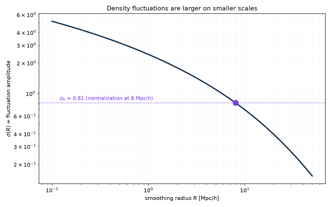
$$\sigma^2(R)=\int_0^\infty\frac{dk}{2\pi^2}\,k^2\,P(k)\,|W(kR)|^2,$$

with $W$ a window function. Evaluated at $R=8\,h^{-1}$Mpc this is $\sigma_8$; as a function of mass it is $\sigma(M)$ (second figure), the quantity the halo mass function depends on. Because there is more power on small scales, $\sigma$ rises as $M$ falls — small halos are common, giant ones rare.

Worked example — what mass does σ₈ probe?

The $8\,h^{-1}$Mpc sphere encloses $M=\tfrac{4}{3}\pi\bar\rho_m R^3$ with $\bar\rho_m=\Omega_m\times2.775\times10^{11}=8.6\times10^{10}\,M_\odot h^{-1}(h^{-1}{\rm Mpc})^{-3}$, so

$$M=\tfrac{4}{3}\pi(8.6\times10^{10})(8)^3\approx1.5\times10^{14}\ M_\odot/h.$$

So $\sigma_8=0.81$ is the fluctuation amplitude on cluster scales. On dwarf-galaxy scales ($\sim10^{9}\,M_\odot$) $\sigma$ is several times larger — which is why such halos are so numerous in CDM, and exactly the population FDM wipes out.

$\sigma(R)$ from the same $P(k)$: the fluctuation amplitude rises toward smaller scales. The marked point at $8\,h^{-1}$Mpc is $\sigma_8$, the standard normalization.

Why P(k) is the master quantity

Everything flows from $P(k)$: growth scales it by $D^2(a)$; the transfer function (Topic 6) shapes it; $\sigma(M)$ integrates it; the halo mass function (Topic 7) is built from $\sigma(M)$; and the FDM cutoff is simply a modification of $P(k)$ at large $k$. Get $P(k)$ right and the rest follows.

In our research

Our entire Task-1 pipeline is an operation on $P(k)$: build it from the Eisenstein–Hu $\times$ Hu–Barkana–Gruzinov transfer, normalize to $\sigma_8$, integrate to $\sigma(M)$, feed Press–Schechter. The FDM suppression is a cutoff imprinted on this $P(k)$; the mandatory sharp-$k$ window (Topic 6.4) exists precisely because that cutoff removes the small-scale power a top-hat would still count.

Key references

Peebles (1980), The Large-Scale Structure of the Universe.
Dodelson & Schmidt (2020), Modern Cosmology, 2nd ed.

PreviousLinear perturbations and the growth of structure NextCosmic epochs relevant to our work (z=127→0)