Computing a soliton: imaginary-time relaxation

The soliton has no closed form, so we compute it. The standard trick — evolving the Schrödinger equation in imaginary time — turns quantum evolution into a relaxation that slides any starting guess down to the ground state. This is the numerical method behind our validated core.

The imaginary-time idea

Replace $t\to-i\tau$ in the Schrödinger equation. The oscillating phase factors $e^{-iE_nt/\hbar}$ become decaying exponentials $e^{-E_n\tau/\hbar}$, so higher-energy components die away faster than the ground state. Renormalizing the wavefunction after each step, any initial guess (with the right symmetry) relaxes to the lowest-energy state — the soliton.

The algorithm

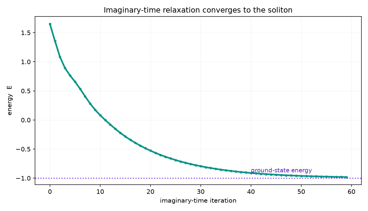
Concretely: (1) start from a trial $\psi$; (2) take a small imaginary-time step of the SP evolution, solving Poisson for $\Phi$ each step; (3) renormalize to fixed mass; (4) repeat until the energy stops changing (figure). Because excited-state contamination decays exponentially, convergence is fast and robust.

Worked example — the convergence test we use

We iterate until the fractional energy change per step falls below a tolerance (e.g. $|\Delta E/E|<10^{-8}$). At convergence the JAXiON solver reproduces the Schive profile to $<1\%$ and the $\rho_c r_c^4$ invariant to five significant figures — the validation (JXE-F5) that licenses using the solver for cores of all masses via the scaling symmetry.

Imaginary-time relaxation: the energy decreases monotonically from an arbitrary initial guess to the ground-state value (dashed) — the soliton. Higher-energy contamination decays exponentially.

Why it is the right tool

Imaginary-time relaxation is variational: it monotonically lowers the energy, so it cannot overshoot or oscillate around the answer. It naturally enforces the nodeless ground state (excited, node-bearing states are higher energy and decay away), exactly the soliton we want.

Differentiability

Because the whole relaxation is a sequence of differentiable operations, one can propagate gradients through it — computing how the soliton (and any observable built from it) changes with the boson mass. This is the foundation of our differentiable inference pipeline (Topic 9.6): the solver is not just a calculator but a differentiable model.

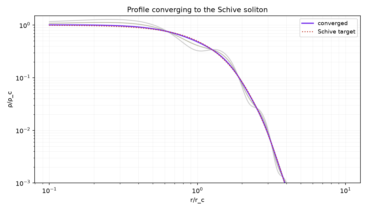
The profile converging onto the Schive soliton as imaginary-time relaxation proceeds.

In our research

This is exactly how our JAXiON soliton solver works (JXE-F5): imaginary-time relaxation reproducing the Schive profile to $<1\%$. Its differentiability is what enables the gradient-based boson-mass inference (Topic 9.6, our differentiable-SBI novelty), and the scaling symmetry (Topic 4.3) then extends one converged solve to every core mass.

Key references

Chavanis (2011), Phys. Rev. D 84, 043531.
Schive, Chiueh & Broadhurst (2014), Nature Physics 10, 496 (arXiv:1406.6586).
Edwards et al. (2018), PyUltraLight, JCAP 10, 027 (arXiv:1807.04037).

PreviousA soliton inside a halo: core + envelope NextGrowth of perturbations and the growth factor