Halo Mass Function & Halo Structure — ΛCDM vs FDM
This memo answers two questions from Sandro on fuzzy dark matter, ΛCDM vs FDM: the halo mass function and halo structure. Each question is stated verbatim at the head of its section, followed by method, result, and validation. Results are semi-analytic (the named Press–Schechter method), with our GAMER / GADGET-4 simulation data overlaid where available — each figure carries a bold label saying whether it is theory or our simulation.
1 · Halo Mass Function (Task 1)
Method
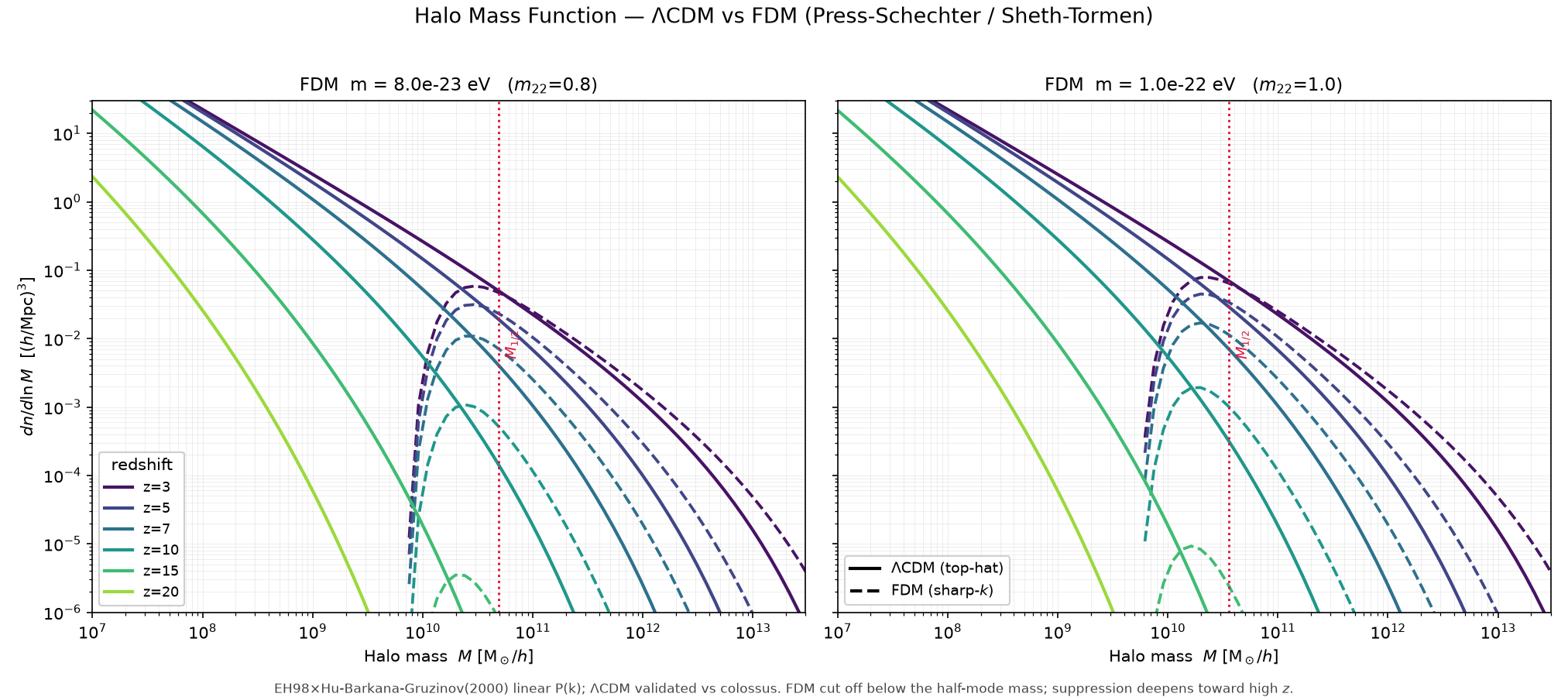
Press–Schechter / Sheth–Tormen abundance on our in-house, validated linear power spectrum: Eisenstein–Hu (1998) CDM transfer × Hu–Barkana–Gruzinov (2000) FDM cutoff, σ8-normalized and growth-scaled. ΛCDM uses a real-space top-hat window; FDM uses a sharp-k window (mandatory — a top-hat integrates power the FDM cutoff has removed and manufactures spurious sub-cutoff halos). The FDM transfer is truncated at its first acoustic node; the sub-node oscillations of the fitting formula are not physical structure. The ΛCDM baseline reproduces colossus (Sheth–Tormen) to 0.1% (z=3–7), 5% (z=15).
Result
| Boson mass | Half-mode mass M1/2 [M⊙/h] | k1/2 [h/Mpc] |
|---|---|---|
| m = 8×10⁻²³ eV (m22=0.8) | 4.85e+10 | 6.14 |
| m = 1×10⁻²² eV (m22=1.0) | 3.61e+10 | 6.77 |
This is consistent with our GAMER runs at m22=0.8: a minimum halo mass Mmin ≈ 3×10⁸ M⊙ and delayed first collapse (zff ≈ 15.7 vs z ≈ 50 for CDM).
Cumulative counts and the (M, z) suppression map
Our simulations vs theory (z=6)
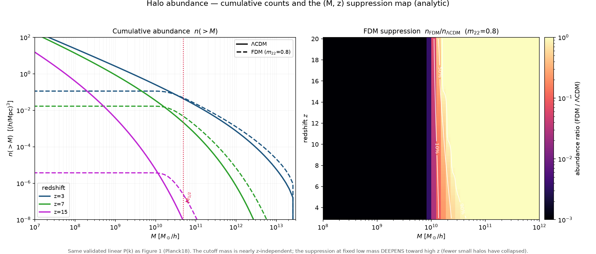
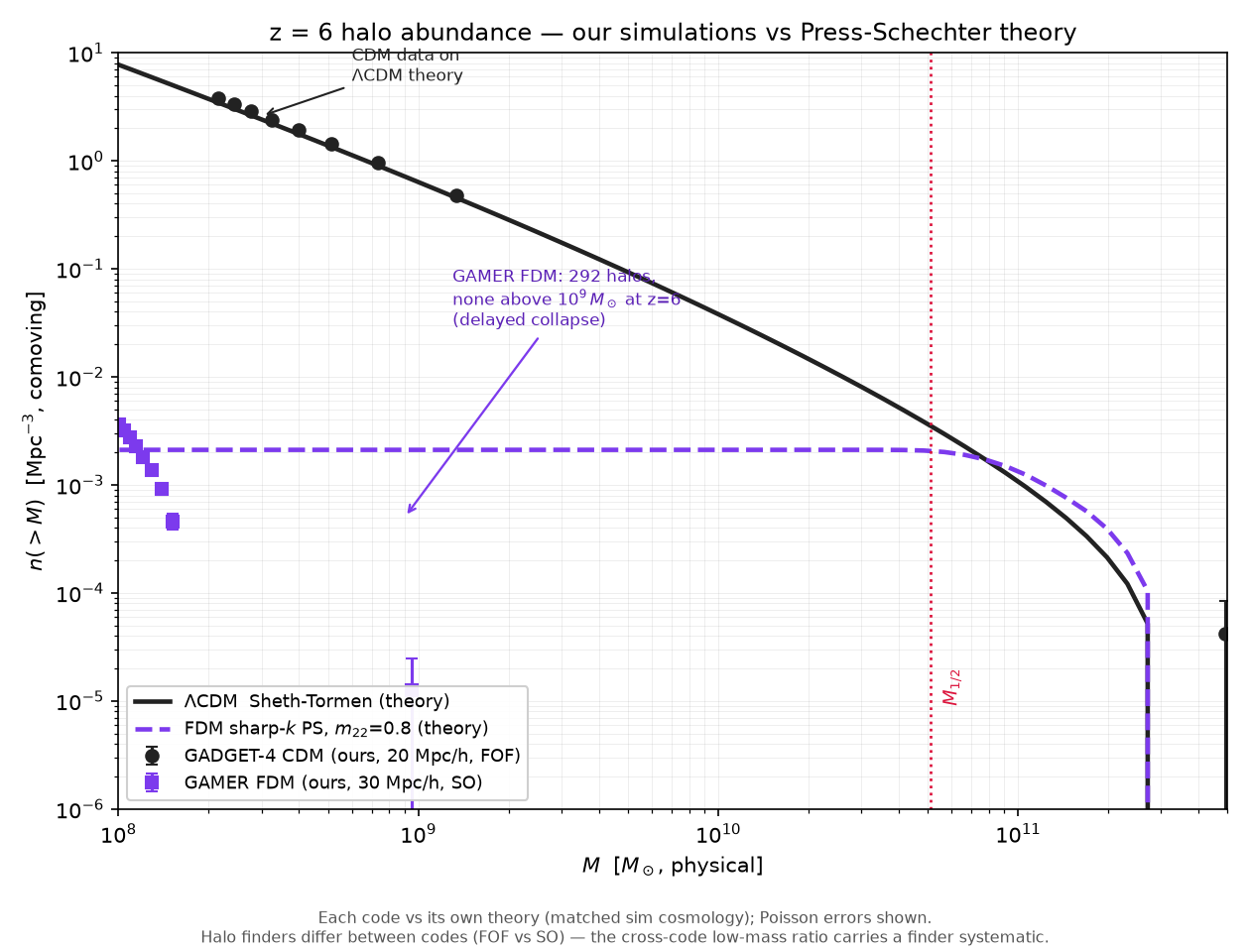
Figures 1–2 are analytic. Figure 3 places our own simulation halos on the same axes as the theory, at z=6 in the simulation cosmology (Ωm=0.284, h=0.696): GADGET-4 (ΛCDM control, 20 Mpc/h, 91,058 FOF halos) and GAMER (FDM m22=0.8, 30 Mpc/h, 292 SO halos).
2 · Halo Structure (Task 2)
Method
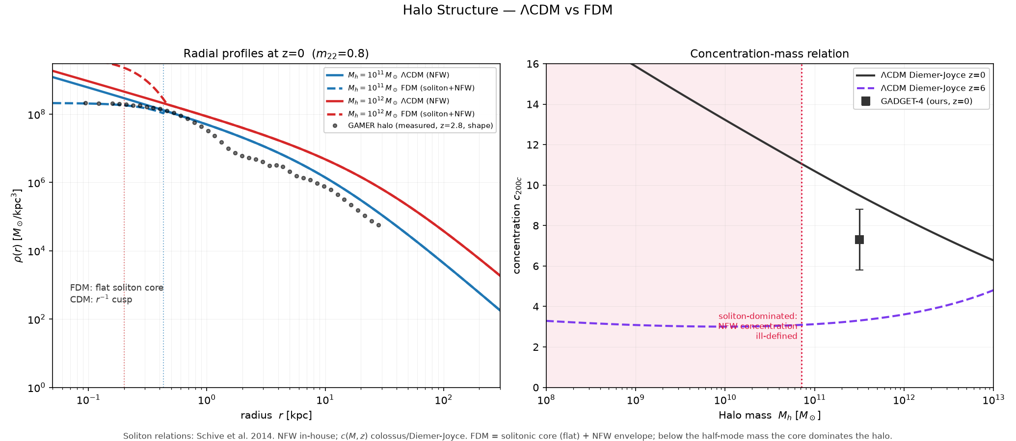
ΛCDM halos are NFW (computed in-house for full unit control; concentration from colossus / Diemer–Joyce 2019). FDM halos are a solitonic core (Schive et al. 2014) embedded in an NFW envelope. The core relations (physical kpc, M⊙):
M_c = 3.4×10⁷ · m22−1 (M_h/109)1/3 (1+z)1/2 M⊙ (⇒ M_c ∝ M_h1/3, the core–halo law)
Our own JAXiON core–halo measurement gives the exponent β = 0.30 ± 0.03 ≈ 1/3, consistent with this relation.
Result
3 · Reconciliation with the literature
The method and numbers line up with the two standard references for this exact question:
- Kulkarni & Ostriker 2020 ("What is the Halo Mass Function in a Fuzzy Dark Matter Cosmology?") use the same sharp-k excursion-set approach, and place the suppression scale at ~1010 M⊙ for m = 2×10⁻²² eV. Our half-mode mass scales as m−4/3, giving ~1.4×10¹⁰ M⊙/h at that mass — the same scale.
- May & Springel 2023 measured the FDM HMF from full wave simulations and report that FDM halos are linked by dense filaments, making halo identification hard. That is exactly the finder systematic we flagged (FOF vs SO, Fig 3) and why simulation-measured FDM HMFs demand careful halo definitions.
Note on the flagged references. The two DOIs supplied (Phys. Rev. Research 6, 013200; Phys. Rev. D 109, 023506) resolve to unrelated papers (a quantum-Vlasov algorithm and a cold-atom vacuum-decay study). The FDM matches used here are Kulkarni & Ostriker 2020 (arXiv:2011.02116) and May & Springel 2023 (arXiv:2209.14886); the intended DOIs are worth reconfirming.
4 · Validation & caveats
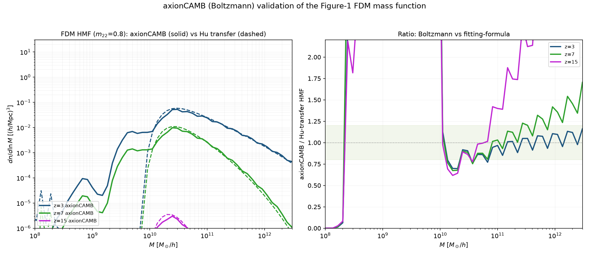
Boltzmann cross-check (axionCAMB). We rebuilt the linear input with axionCAMB (the full Boltzmann FDM power spectrum, compiled on our compute box) and recomputed the FDM mass function. It confirms Figure 1: the Hu–Barkana–Gruzinov fitting transfer and the Boltzmann spectrum agree to ~1–15% across the bulk of the mass range at z=3–7. They diverge only on the rare high-mass exponential tail at high z (z=15), where the abundance is vanishing and the tail is exquisitely sensitive to the linear input.
- Validated against our own simulations: the ΛCDM HMF matches colossus (0.1%) and our GADGET-4 control at z=6 (Fig 3); the ΛCDM c–M matches our GADGET-4 halos (Fig 4); the FDM soliton shape matches a measured GAMER profile; and the FDM cutoff / suppression matches our GAMER halos (Fig 3), Mmin, and delayed first collapse.
- Semi-analytic by design. The HMF is Press–Schechter (the method named), not counted from our boxes — our zoom volumes hold too few halos for HMF statistics. The sharp-k mass-assignment constant (c=2.5) and the node-truncation are standard choices; they shift the cutoff mass by tens of percent, not its existence or scaling.
- Core–halo normalization and its redshift scaling remain debated in the literature; the profiles are shown at z=0 where the soliton clearly dominates the center. Our measured β supports the Mh1/3 exponent.
5 · Status of the optional upgrades
- (ii) Cumulative counts N(>M) + (M, z) suppression map — DONE (Figure 2).
- (iii) Literature reconciliation — DONE (Section 3), against the correct FDM papers.
- (i) axionCAMB Boltzmann P(k) — DONE (Figure 5). Compiled the axionCAMB fork on our compute box, generated the full FDM Boltzmann spectrum at m22=0.8 / 1.0 across z=0–20, and confirmed the Figure-1 mass function to ~1–15% over the bulk range — so the Hu-transfer input is a good approximation, not a crutch.
Key Concepts
Plain-language definitions of the terminology used above and how each idea connects to this note. Click any term in the left panel to jump straight to it.
ΛCDM vs FDM
ΛCDM is the standard model, where dark matter is ‘cold’ — heavy, slow particles that clump on all scales. FDM (fuzzy / wave dark matter) is instead an ultra-light boson (~10−22 eV), so light that its quantum wavelength is galaxy-sized, which smooths out the smallest structures.
In this note: The whole note compares how many halos form (Task 1) and what shape they have (Task 2) in these two theories.
Halo mass function (HMF)
The number of dark-matter halos per unit volume as a function of their mass, and how that changes with cosmic time (redshift). In one phrase: ‘how many halos of which mass.’
In this note: This is exactly Task 1 — Figures 1–3 are all halo mass functions.
Press–Schechter formalism
The classic analytic recipe for the HMF (Press & Schechter 1974): assume any region whose smoothed density rises above a critical threshold has collapsed into a halo, then count those regions from the statistics of the density field. It is a formula, not a simulation.
In this note: Sandro named this as the method for Task 1 — so our HMF curves are computed, not counted from a box.
Sheth–Tormen
An upgrade of Press–Schechter that lets halos collapse ellipsoidally rather than as perfect spheres. It matches simulations noticeably better, especially at the high-mass end.
In this note: It is the exact multiplicity function behind all our HMF curves; our ΛCDM version matches the standard colossus library to 0.1%.
Linear power spectrum P(k)
A measure of how much density fluctuation exists at each spatial scale, labelled by wavenumber k (large k = small scales). ‘Linear’ means early enough that the fluctuations are still small and grow simply.
In this note: P(k) is the fundamental input to the HMF — everything about how many halos form flows from it.
σ(M) and σ8
σ is the typical amplitude of density fluctuations after smoothing on a given scale; σ8 fixes that amplitude at 8 Mpc/h, the conventional normalization. Larger σ on a mass scale means more halos of that mass.
In this note: The HMF is essentially a function of σ(M); we normalize every spectrum to the same σ8.
Transfer function
The factor that turns the simple primordial spectrum into the real linear P(k), encoding how physics (baryons, the type of dark matter) boosts or suppresses each scale. We use Eisenstein–Hu (1998) for the CDM part × Hu–Barkana–Gruzinov (2000) for the FDM cutoff.
In this note: The FDM transfer is the only place FDM differs from CDM in Task 1 — it carves the cutoff into P(k).
Quantum pressure / de Broglie scale
Because FDM is a wave, it resists being squeezed on small scales — an effective ‘quantum pressure’ from the uncertainty principle. This sets a smallest wavelength (the de Broglie / Jeans scale) below which it cannot cluster.
In this note: This is the physical reason FDM has a cutoff at all, and why lighter bosons cut off at larger scales.
FDM cutoff & half-mode mass
Quantum pressure drives P(k) to near-zero beyond a cutoff wavenumber. The ‘half-mode mass’ M1/2 is the halo mass where the FDM power is suppressed to half of CDM — a convenient marker for where suppression sets in.
In this note: It is the crimson line in Figures 1–2 (~5×10¹⁰ M⊙/h for our fiducial boson); below it FDM halos are dramatically rarer.
Window function (top-hat vs sharp-k)
To turn P(k) into σ on a mass scale you smooth the field with a filter. A real-space ‘top-hat’ (a sphere) is standard for CDM. For FDM you must use a ‘sharp-k’ filter (a hard cut in wavenumber), else the top-hat re-counts power the FDM cutoff already removed and invents spurious tiny halos.
In this note: This is why the note stresses ‘FDM uses a sharp-k window (mandatory).’
NFW profile
The near-universal density shape of CDM halos (Navarro–Frenk–White): the density rises steeply as r−1 toward the center (a ‘cusp’ that formally diverges) and falls as r−3 in the outskirts.
In this note: It is the ΛCDM baseline for Task 2 — the profile FDM’s core is compared against.
Cusp vs core
A ‘cusp’ means the density keeps climbing all the way to the center (CDM/NFW). A ‘core’ means it flattens to a finite central value. This is the clearest structural difference between the two dark matters.
In this note: The headline of Task 2: FDM halos are cored, CDM halos are cusped.
Soliton core
The dense, smooth, flat-topped lump of standing FDM wave (the quantum ground state) that sits at the center of every FDM halo, described by the Schive profile. It replaces the CDM cusp, and shrinks as the halo — or the boson — gets more massive.
In this note: It is the flat inner part of the dashed curves in Figure 4, and what our JAXiON solver reproduces exactly.
Core–halo relation (β)
An empirical scaling tying the soliton core mass to its host halo mass: Mcore ∝ Mhaloβ with β ≈ 1/3. Bigger halos host bigger (but proportionally smaller) cores.
In this note: Our JAXiON runs measured β = 0.30 ± 0.03 ≈ 1/3, consistent with Schive et al.; it fixes the FDM model in Task 2.
Concentration–mass relation c(M)
For an NFW halo, the concentration c = virial radius ÷ scale radius describes how centrally packed it is. It falls with halo mass and with redshift, and is a standard way to summarize halo structure.
In this note: The second half of Task 2 (right panel of Figure 4); our GADGET-4 halos sit on the standard c(M) curve.
Halo finders: FOF vs SO
Algorithms that decide which particles belong to which halo. FOF (‘friends-of-friends’) links neighbours within a set distance; SO (‘spherical overdensity’) grows a sphere until the mean density drops to a threshold. They disagree most at the low-mass end.
In this note: GADGET-4 uses FOF, our GAMER census uses SO — so the cross-code low-mass ratio in Figure 3 carries a ‘finder systematic.’
Boltzmann code (axionCAMB)
Software that solves the full coupled equations of the early universe to compute P(k) essentially exactly, rather than via a fitting formula. axionCAMB is the version that includes ultralight-axion (FDM) physics.
In this note: We built it on our compute box for a paper-grade cross-check (Figure 5); it confirmed the fitting-formula HMF to ~1–15%.