fdmsim · quantum simulation program

Two Frontiers of Quantum Simulation

Two 2024 papers, reproduced & extended — the analog face (mimic the physics with a stand-in physical system) and the digital face (run it as a quantum circuit) of quantum simulation, both on one core engine: our differentiable spectral solver.

VACUA · vacuum decay in a cold-atom BEC
Jenkins et al., PRD 109, 023506 (2024)
The paper · mechanism
Analog · cold-atom experiment (their proposal)
What we did · our reproduction
Numerical simulation (classical spectral)
1
Two-component BEC
⁴¹K condensate of two atomic states; relative phase φ is the field.
1
Differentiable spectral split-step solver
Same FFT engine as our FDM code.
2
Modulated coupling (λ) → false-vacuum well
An rf drive sculpts the double-well potential.
2
Seed the correct quantum jitter
Bogoliubov-correlated fluctuations — not plain random noise.
3
Fluctuations → bubble
Nucleates and expands relativistically.
3
Evolve the two-field GPE
Bubble nucleates & expands at 45° (relativistic).
4
Image the condensate
Read out the relative phase to watch the decay.
4
Fit the decay rate Γ(n̄)
Matches the paper's theory.
Runs on — a cold-atom BEC (analog)
Proposed platform, not built yet. The paper's own figures are classical numerics.
Runs on — an ordinary classical computer
Our spectral solver; no quantum hardware.
QVLASOV · quantum algorithm for neutrino structure
Miyamoto et al., PRR 6, 013200 (2024)
The paper · algorithm
Digital quantum algorithm
What we did · our reproduction
Numerical simReal IonQ hardware
1
Linearize Vlasov
Drop neutrino self-gravity → the equation becomes linear.
1
Classical Vlasov reference
scipy matrix-exp — the ground truth.
2
Recast as Schrödinger (H = iA)
i∂ₜ|f⟩ = H|f⟩, with A antisymmetric.
2
Trotterize + exact statevector emulation
4–6 qubits, noiseless.
3
Qubits + Trotter
Load f into amplitudes; split e^(−iHt) into gate steps.
Would require a fault-tolerant machine: a logarithmic number of error-corrected logical qubits + a QRAM (O(n_gr³) entries). A realistic 6-D cosmological run → thousands of physical qubits + QRAM that doesn't exist yet.FTQC · not today's hardware
3
Transpile → real IonQ Forte-1
4 physical NISQ qubits, 300 shots, no error correction — the core mechanism at toy scale (n_gr = 4), not the full algorithm.
Quantum hardware
4
Run the circuit → power spectrum
Measure, reconstruct the neutrino power spectrum.
4
Benchmark classical ↔ simulator ↔ hardware
And root-cause the noise.
Runs on — fault-tolerant QC + QRAM (digital)
Proposed platform, not built yet. Paper's own figures are classical numerics.
Runs on — classical + real IonQ Forte-1 qubits
The one place real quantum hardware enters this program.
The gap: the paper's full algorithm needs a fault-tolerant machine (thousands of logical qubits + QRAM); we ran its core mechanism on 4 real NISQ qubits — a faithful toy, not the full speedup.
Deck · 20 Jul 2026 · use ← / → to navigate
Paper 1 · VACUA · the physics

False-vacuum decay, on a tabletop

Quantum nucleation of true-vacuum bubbles from a metastable "false vacuum" — the early-universe process behind eternal inflation, electroweak baryogenesis, Higgs metastability and gravitational-wave backgrounds — realized as an analog in a two-component ⁴¹K Bose–Einstein condensate.

  • The condensate's relative phase φ obeys a relativistic Klein–Gordon equation (a relativistic wave equation) in a double-well potential.
  • The "speed of light" is the sound speed c = √(gn/m) ≈ 6 mm/s — relativity, at walking pace.
  • A metastable well at φ = π appears only when the modulation λ > 1; below that it vanishes.
U(φ) = 4εφ02 (m2c2/ℏ2) [ 1 − cos(φ/φ0) + ½ λ2 sin2(φ/φ0) ] Jenkins+24, Eq. 10 — λ is the knob that carves the middle dip.
  • φ — the field: the relative phase between the two BEC species (the ball's position on the landscape).
  • φ₀ — the yardstick: a fixed scale (√(ℏ²n/2m)); we plot φ/φ₀, so vacua land at 0, π, 2π…
  • λ — the knob: the modulation strength that shapes the landscape; λ>1 creates the false-vacuum dip.
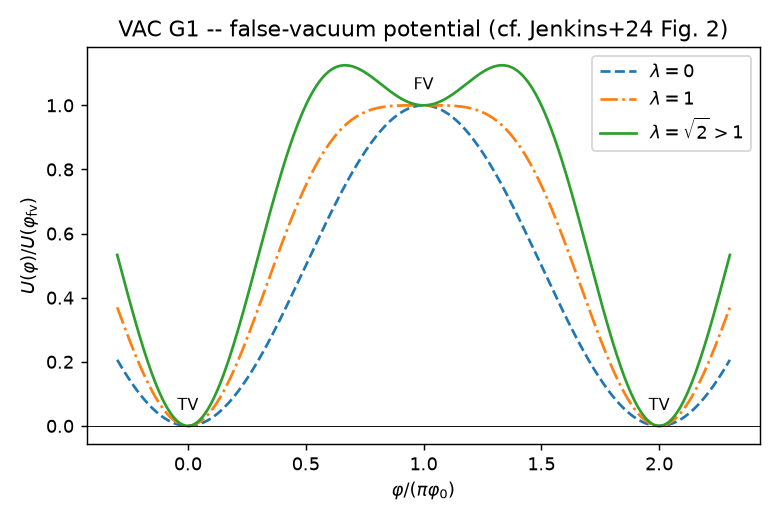
false-vacuum double-well potential
Fig. 2 — the false-vacuum landscape: metastable minimum at φ=π for λ>1.
Paper 1 · VACUA · simulation approach

Spectral split-step + the correct quantum vacuum

We evolve the condensate with our own spectral split-step solver (the same engine as our FDM code — no new machinery). The hard part isn't evolving the field; it's how you start it.

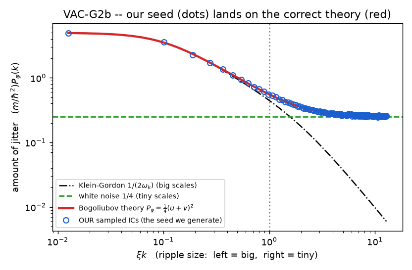
  • You must seed the correct quantum jitter. Even a "resting" vacuum trembles; the simulation must start from that exact tremor pattern — strong at large scales, flat at tiny scales.
  • The lazy shortcut fails. Seeding plain random noise makes the vacuum decay too fast (it's secretly an excited state) — a fake, inflated result. The paper flags this as the easy-to-botch step.
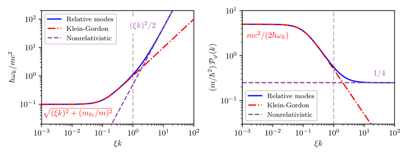
  • This chart is the receipt. It checks our starting jitter is right — and it is.
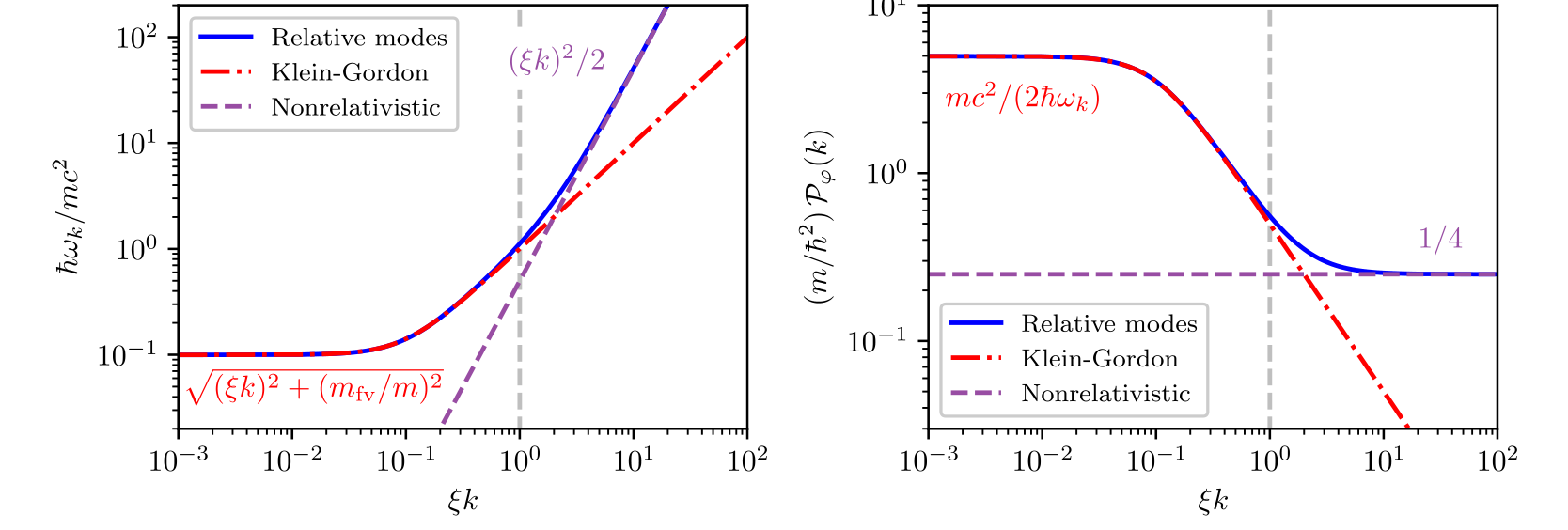
THE PAPER — Jenkins+24, Fig. 3. Right panel: the fluctuation spectrum — Klein–Gordon at big scales, flat "white noise" (¼) at tiny scales.
Jenkins Fig 3 dispersion and spectrum
OURS — the same spectrum (right panel), reproduced.
our Bogoliubov spectrum reproduction
The point: our sampled starting conditions (circles) land on the correct theory curve — matched to 0.1% — reproducing the paper's right panel. It is not flat: it bends at the healing scale, so naïve "white noise" would be visibly wrong. This quality gate makes the bubble & decay-rate results trustworthy.
Paper 1 · VACUA · results in the paper

Bubbles nucleate; the rate obeys the theory

Jenkins et al. demonstrate quantum-regime false-vacuum decay in a two-component ⁴¹K condensate — an Editors' Suggestion in Phys. Rev. D. The headline: the decay rate is set by the fluctuation amplitude, exactly as the instanton theory predicts.
Editors' Suggestion PRD 109, 023506 (2024) T ≲ 10.9 nK charges ~ppb
Jenkins et al. Figure 6 from the paper
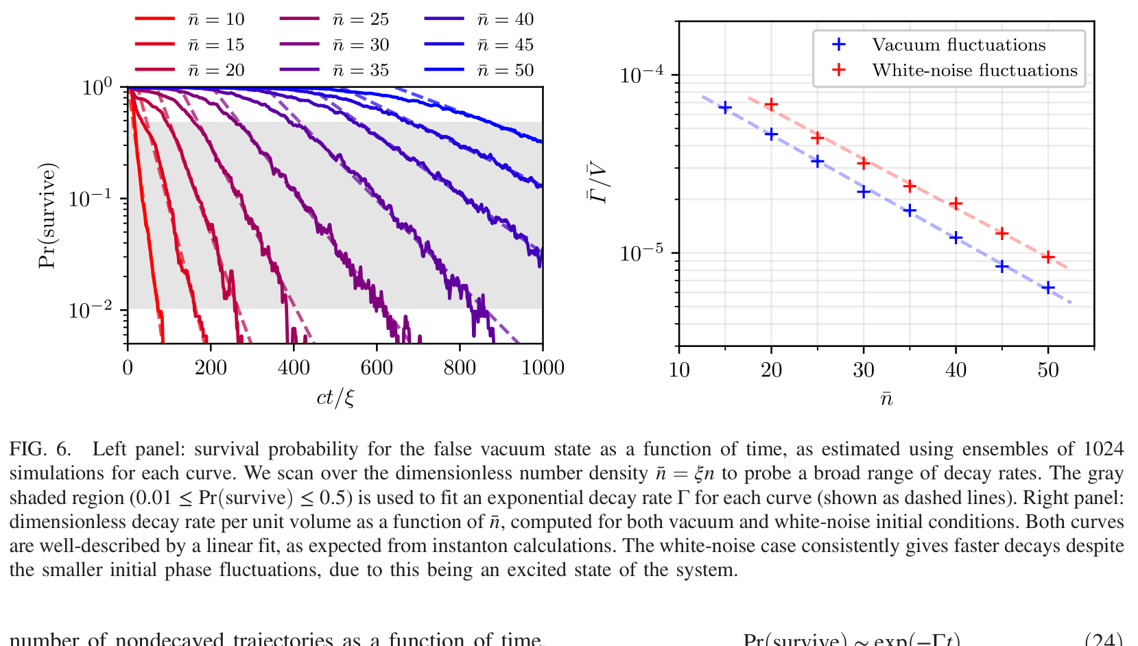
The paper — Jenkins+24, Fig. 6
  • Sweeps amplitude n̄ = 10–50, 1024 simulations per point.
  • Left: survival P(t) ~ exp(−Γt). Right: decay rate Γ/V falls steeply as n̄ grows.
  • Vacuum (blue) decays slower than white-noise (red) — white noise is an excited state that over-nucleates.
  • The rate is set by the fluctuation amplitude, exactly as instanton theory predicts (Eq. 22).
our reproduction: decay rate vs amplitude
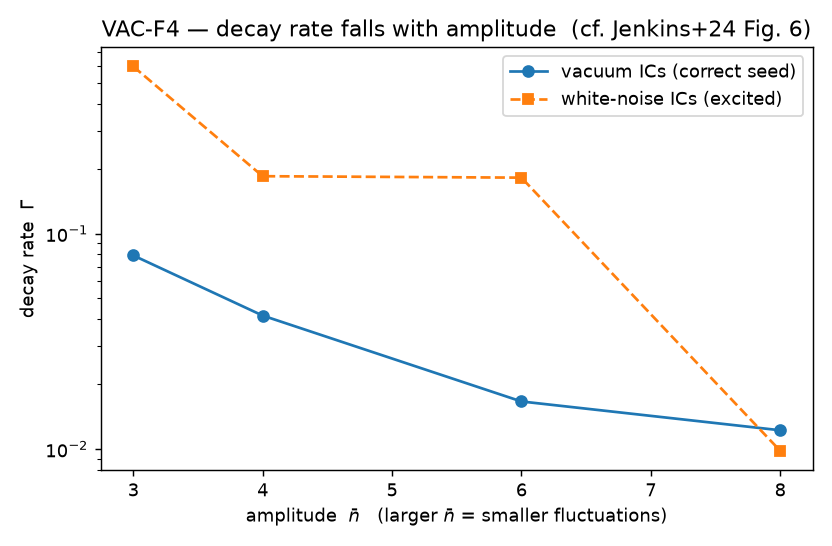
Ours — reproduced on our engine
  • The same measurement: Γ vs n̄, vacuum (blue) vs white-noise (orange).
  • Both trends reproduced: Γ falls with n̄, and white-noise decays faster.
  • Honest differences: n̄ = 3–8 (a cheaper laptop slice), fewer samples, different normalization — trends match, not an exact overlay.
  • The full n̄ = 10–50 GPU reproduction is queued.
Paper 1 · VACUA · what we reproduced

A bubble nucleating, on our own engine

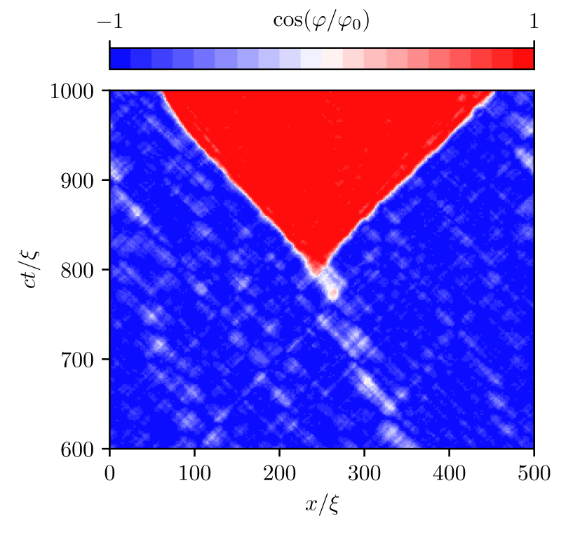
Blind, check-by-check reproduction (G0–G4) on our differentiable spectral solver — the money shot: a true-vacuum bubble whose wall expands at 45°, i.e. at the phonon "speed of light."
Jenkins Fig 1 bubble nucleation
The paper — Jenkins+24, Fig. 1
  • A space-time diagram: time runs up, position across, colour = which vacuum each point sits in.
  • A true-vacuum bubble (red) nucleates out of the fluctuating false vacuum (blue).
  • Its walls expand at 45° — the phonon "speed of light" — exactly as vacuum-decay theory predicts.
  • Run on their cold-atom analog model (2048-site lattice).
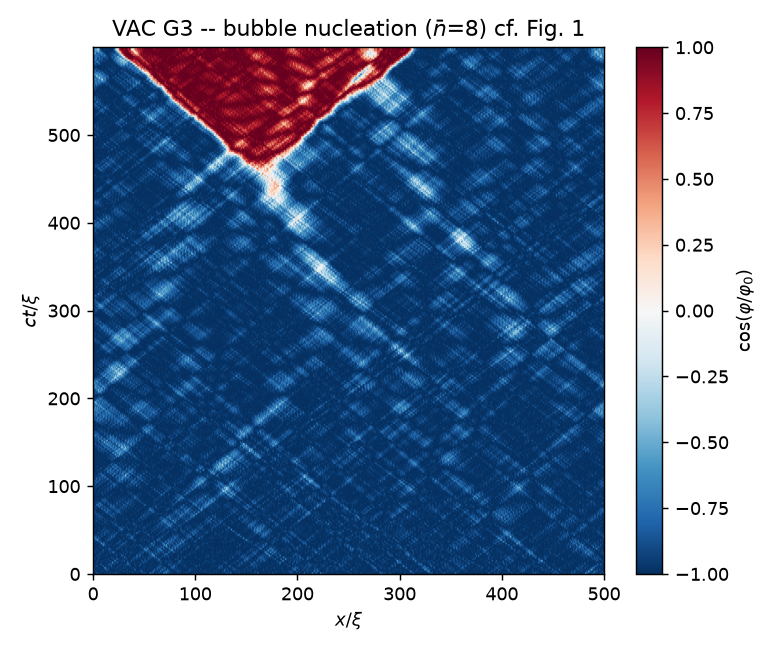
our space-time diagram of bubble nucleation
Ours — reproduced on our engine
  • Blind, check-by-check (G0–G4) on our differentiable spectral solver.
  • A bubble nucleates (~ct 450) and its wall races out at the identical 45°.
  • Engine checks: conserved quantities hold to 3×10⁻¹²; the correct quantum-jitter start to 0.1%.
  • Honest: reduced-statistics laptop run (N=1024) — same phenomenon, our own run beside the paper's.
Paper 2 · QVLASOV · the physics

Massive neutrinos as hot dark matter

Neutrinos have tiny mass but huge velocities — hot dark matter that shapes cosmic large-scale structure differently from cold dark matter. Observing that structure constrains the neutrino mass.

  • Because they fly freely (free-streaming), they wash out structure below a characteristic size.
  • To predict that, you must track their full spread over both position and velocity — the 6-D distribution f(x, v).
  • The neutrino mass is one of the last unmeasured Standard-Model numbers — cosmology is the sharpest probe.
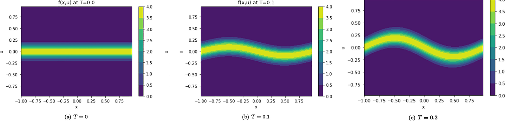
THE PAPER — Miyamoto+24, Fig. 2. Phase space f(x,v) at three times — the calm band shears as gravity acts.
Miyamoto Fig 2 phase space (three panels in a row)
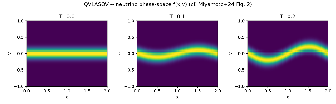
OURS — the same phase-space evolution, reproduced.
our neutrino phase space distribution
Reading both: position across, velocity up, colour = how many neutrinos at each position-and-speed. The distribution starts as a flat band and shears under gravity — this whole object is what the simulation evolves. Our run reproduces the paper's.
Paper 2 · QVLASOV · simulation approach

From Vlasov to a quantum circuit

The Vlasov equation isn't quantum — but a few honest approximations turn it into exactly the kind of problem a quantum computer is built to solve. Follow the chain:

1

Linearize the physics

Neutrinos are <1% of all matter, so ignore their own gravity and treat the dark-matter pull as a fixed external force. With that, the Vlasov equation becomes linear.

∂f/∂t + v·∂f/∂x + FCDM·∂f/∂v = 0  (Eq. 4)

2

Rewrite it as a Schrödinger equation

Put the distribution f on a grid and the equation becomes df/dt = A·f with A antisymmetric. Multiply by i and it is literally a Schrödinger equation — a cosmology equation in disguise as quantum mechanics.

i ∂t|f⟩ = H|f⟩,  H = iA  (Hermitian)

3

Load f into qubits

Store the grid of numbers in the amplitudes of qubits. n qubits hold 2ⁿ grid points — so the 6-D phase-space explosion becomes "a few more qubits," not exponentially more memory. This is where the quantum advantage comes from.

n qubits → 2ⁿ grid points

4

Evolve with Hamiltonian simulationthe missing bridge

The answer is |f(T)⟩ = e−iHt|f(0)⟩. A quantum computer can't apply that giant operator in one shot — so split it into tiny alternating steps: a little streaming, a little gravity, repeated. That's Trotterization, and each tiny step is just a small set of standard quantum gates.

|f(T)⟩ = e−iHt|f(0)⟩ ≈ ( e−iHxτ · e−iHvτ )N

5

Run & measure

Those gates form a circuit. Run it, measure the qubits many times, and the measurement statistics reconstruct f(T) → the neutrino power spectrum P(k).

circuit → shots → f(T) → P(k)

Net: a 6-D cosmology PDE → a Schrödinger equation → a gate circuit a quantum computer runs natively. In our QVLASOV lane we actually ran this on IonQ hardware — see slide 10.
Paper 2 · QVLASOV · results in the paper

A quantum algorithm, plus a small demo

This is a quantum-algorithm paper — designed for a future fault-tolerant machine — accompanied by a small classical demonstration of the physics.

  • Small classical demo (Sec. IV): one dimension in position and velocity, a 64-point grid, a single gravity ripple F = A·sin(Kx).
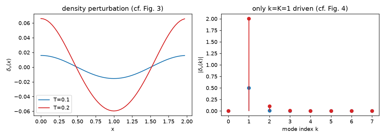
  • That one gravity ripple (wavenumber K) drives only the matching neutrino ripple (k=K) — nothing else (Figs. 3–4).
  • The quantum algorithm scales as Õ(ngr+nt) vs classical O(ngr⁶) — the potential speedup.
  • Reading out the power spectrum (structure vs. size) needs quantum amplitude estimation and a quantum memory (QRAM).
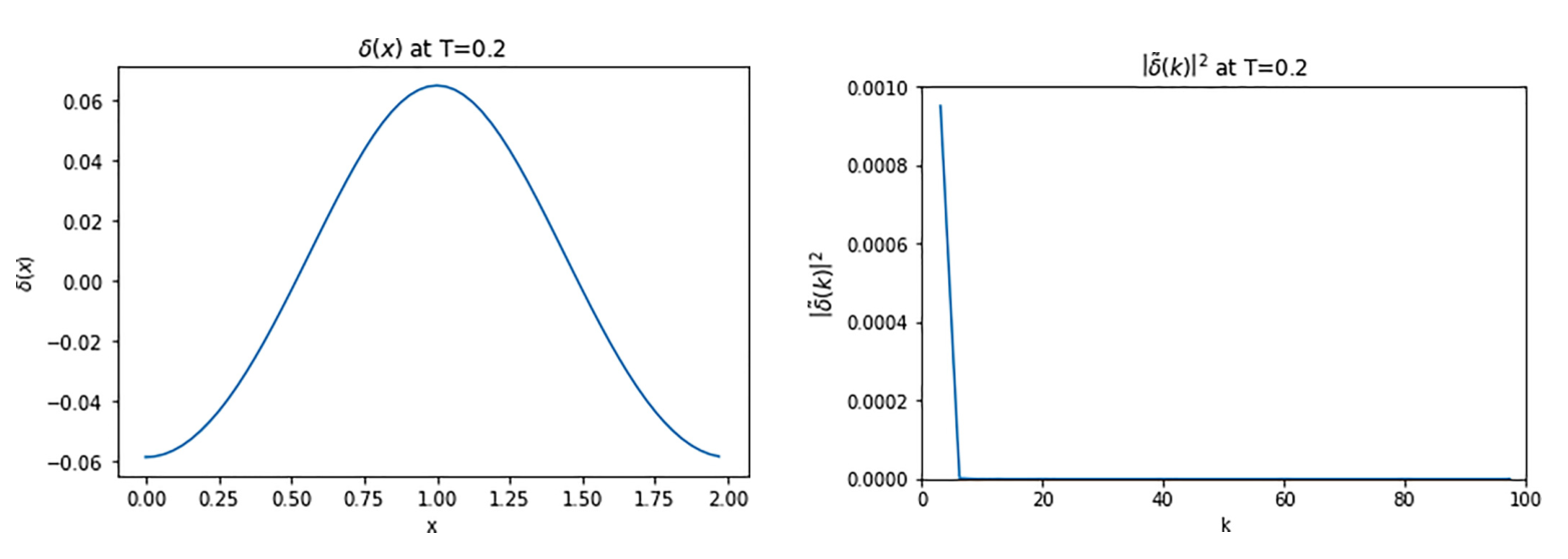
THE PAPER — Miyamoto+24, Figs. 3–4. Left: the neutrino density ripple. Right: its spectrum — a single spike at k=K.
Miyamoto Figs 3-4 density and Fourier mode
OURS — the same single-mode response, reproduced.
our density perturbation, only k=K mode driven
Reading both: feed in one gravity ripple (wavenumber K) and exactly one matching neutrino ripple responds — everything else stays zero. The clean single-mode result the demo is meant to show; ours reproduces the paper's.
Paper 2 · QVLASOV · what we reproduced — and extended

We ran it on real quantum hardware

Beyond reproducing the paper, we did what the authors never did: ran the core step on a real quantum computer — IonQ's trapped-ion Forte-1.

  • Reproduced the classical demo (one gravity ripple drives one neutrino ripple; total probability held to 1e-15).
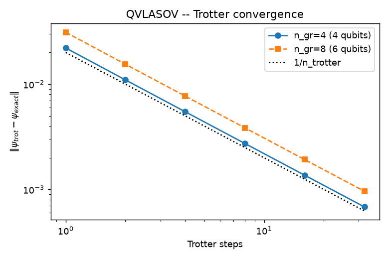
  • The step-by-step (Trotter) version, run on an exact simulator (4–6 qubits), converges to the true answer (top figure).
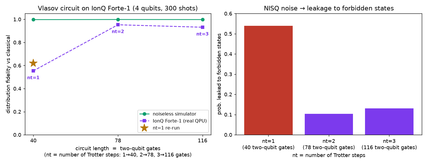
  • Our extension: ran it on IonQ Forte-1 — 4 real qubits, circuits of 40/78/116 two-qubit gates, 300 runs each.
  • Checked classical → cloud simulator (0.996 match) → real machine; when well-calibrated it reproduces the answer to ~90–95%.
Honest ceiling. The full future-hardware algorithm (needs an error-corrected / fault-tolerant machine, a quantum memory / QRAM, 6-D, amplitude estimation) won't run on today's noisy quantum computers — we ran the toy-scale core step, not the asymptotic speedup.
Trotter convergence
Top — the point: the step-by-step (Trotter) error shrinks toward zero as you add more steps, on an exact simulator. The method itself is sound, before any hardware noise.
IonQ fidelity and leakage
Bottom — the point: on real IonQ hardware — how closely the output matches truth (fidelity) and how much probability leaks to wrong states (leakage), across circuit depths. Calibrated circuits reach ~90–95%.
Paper 2 · QVLASOV · questions & our RCA

Why was the shallowest circuit the worst?

Counterintuitively, the fewest-gate circuit was reproducibly the worst (fidelity ~0.6). A root-cause analysis cleanly separated two error regimes.

  • We varied the number of steps nt at the same total evolution time and compared to a random-noise model — that separates the two error types.
  • Random gate noise alone would make the fewest-gate circuit best (model: 0.84) — but on hardware it's the worst.
  • ⇒ the culprit is a systematic (coherent) error in the shallow, large-rotation-angle case — not random depth noise.
  • From nt ≥ 2 the results follow the random-noise trend; the sweet spot is nt=2.
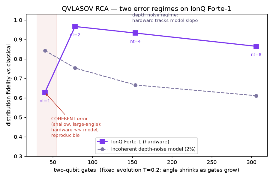
Next: prove the coherent-error mechanism (randomized compiling / error mitigation), push larger ngr on simulator, and find where the quantum speedup actually pays off.
RCA: hardware vs depolarizing noise model
The point of this chart (RCA): real hardware (points) vs a pure random-noise model (line). They disagree exactly where the circuit is shallowest — proof of a systematic error there, not random noise. Two error regimes, cleanly separated.
The big picture · how × what

The Quantum-Simulation Map

Two axes — the method (how) and the phenomenon (what). Most phenomena can be done several ways; each method spans several phenomena. Our two papers sit here ↓; the next slide is the full catalog.

Cold-atom / BECAnalog
Rydberg / lattice arraysAnalog
Superconducting / ionDigital
Fault-tolerant algorithmFTQC · future
Classical numericalClassical
Vacuum decay & the early universe
✓ oursJenkins · VACUAEckelViermann
Black holes & Hawking radiation
Steinhauer '16Steinhauer '19
Benhemou
Shi
Cosmic structure: dark matter & neutrinos
✓ oursMiyamoto · QVLASOV
SchiveMocz
Quantum matter & magnetism
BernienEbadiSemeghiniMazurenko
Arute · FHAndersen · braiding
Lattice gauge theories
Yang
MartinezKokail
Time crystals & non-equilibrium order
Mi
Quantum chemistry & molecules
Kandala · VQEArute · HF
Particle physics & quantum field theory
Klco · SchwingerBauer · partonHall · neutrinos
Jordan–Lee–Preskill
Nuclear physics
Dumitrescu · deuteron
Quantum information: scrambling & holography
Landsman · scrambling
Glowing cells = runs on (or algorithms for) a real programmable quantum computer — Rydberg / optical-lattice arrays, superconducting & trapped-ion processors, and fault-tolerant algorithms. Un-glowed cells are analog-gravity mimicry (cold-atom BEC) or classical numerics. Most are small proof-of-principle demos today.
Analog is the physics; digital & algorithmic compute it; classical is the yardstick — but all reduce to Hamiltonian evolution on a grid.
The wider field · 29 papers

The Quantum Simulation Landscape

Where our two papers sit in the quantum-simulation landscape — 29 papers, analog and digital, from cosmology-in-the-lab to Rydberg arrays, and digital quantum processors running chemistry, high-energy, nuclear & scrambling problems. Our two reproductions are highlighted. Click any chart to enlarge.
Paper
Physics · Approach · Result
Hero chart
Cosmology & curved spacetime, in the lab · analog
Jenkins et al. 2024 — Analog vacuum decay from vacuum initial conditions ✓ reproduced · this deck arXiv 2307.02549 · PRD 109, 023506
PhysicsFalse-vacuum decay / bubble nucleation
ApproachCold-atom BEC, 2-field GPE (analog)
ResultDecay rate Γ set by the correlated-vacuum amplitude; naïve white noise over-nucleates
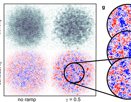
Jenkins vacuum-decay spectra
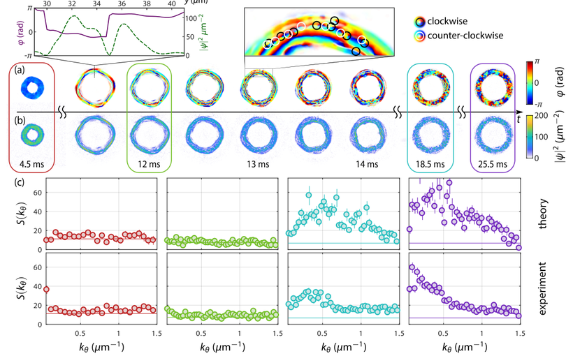
Eckel et al. 2018 — A rapidly expanding BEC: an expanding universe in the lab arXiv 1710.05800
PhysicsExpanding-universe cosmology
ApproachCold-atom BEC, expanding ring (analog)
ResultPhonon redshift + Hubble friction + preheating-like turbulent cascade
Eckel expanding-ring BEC
Viermann et al. 2022 — Quantum field simulator for dynamics in curved spacetime arXiv 2202.10399
PhysicsScalar QFT in curved / expanding spacetime
ApproachCold-atom BEC, tunable 2D metric (analog)
ResultCosmological particle production & Sakharov oscillations in a programmable metric
Viermann curved-spacetime BEC
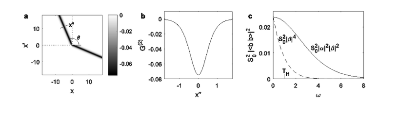
Steinhauer 2016 — Observation of quantum Hawking radiation & its entanglement in an analogue black hole arXiv 1510.00621 · Nat. Phys.
PhysicsHawking radiation (spontaneous, quantum)
ApproachCold-atom BEC sonic horizon (analog)
ResultObserved entangled Hawking–partner phonon pairs across the horizon
Steinhauer 2016 Hawking correlations
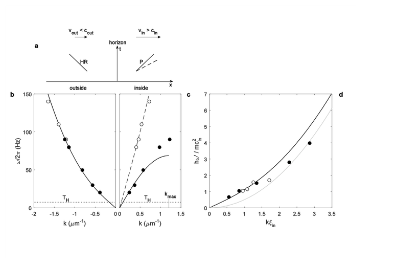
Steinhauer 2019 — Observation of thermal Hawking radiation & its temperature in an analogue black hole arXiv 1809.00913 · Nature
PhysicsHawking radiation thermality & temperature
ApproachCold-atom BEC sonic horizon (analog)
ResultMeasured the Hawking temperature; confirmed a thermal spectrum
Steinhauer 2019 Hawking temperature
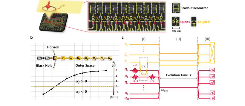
Shi et al. 2023 — Hawking radiation & curved spacetime with a superconducting on-chip black hole arXiv 2111.11092
PhysicsHawking radiation / curved spacetime
ApproachSuperconducting qubit chain, on-chip (analog)
ResultStimulated Hawking-like emission & wave propagation in a curved metric on chip
Shi on-chip black hole
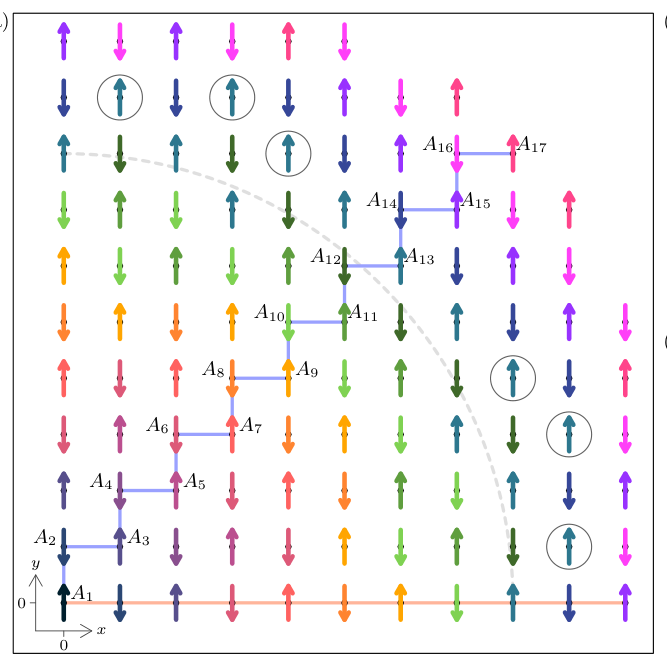
Benhemou et al. 2023 — Probing black holes with a Floquet-driven optical-lattice simulator arXiv 2312.14058
PhysicsAnalog black hole (Hawking, scrambling)
ApproachOptical lattice, Floquet-driven (analog · proposal)
ResultPosition-dependent tunnelling encodes the curved metric; Hawking T from site populations
Benhemou Floquet lattice black hole
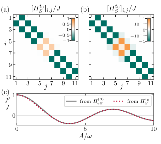
Nixon et al. 2023 — Individually tunable tunnelling in optical lattices via local periodic driving arXiv 2309.12124
PhysicsEngineered lattice Hamiltonians (enabling toolkit)
ApproachOptical lattice, local Floquet driving (analog · theory)
ResultFull local control of tunnelling → SSH / topological & curved-space lattices
Nixon tunable tunnelling
Fuzzy dark matter & neutrino cosmology · numerical / quantum-algorithm
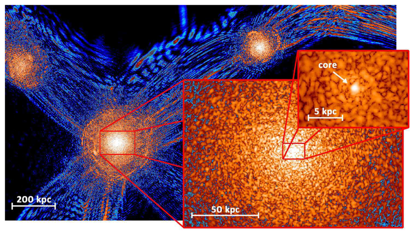
Schive et al. 2014 — Cosmic structure as the quantum interference of a coherent dark wave arXiv 1406.6586 · Nat. Phys.
PhysicsFuzzy dark matter cosmic structure
ApproachClassical spectral Schrödinger–Poisson
ResultSolitonic core in every halo; boson mass mB ≈ 8×10⁻²³ eV
Schive FDM cosmic structure
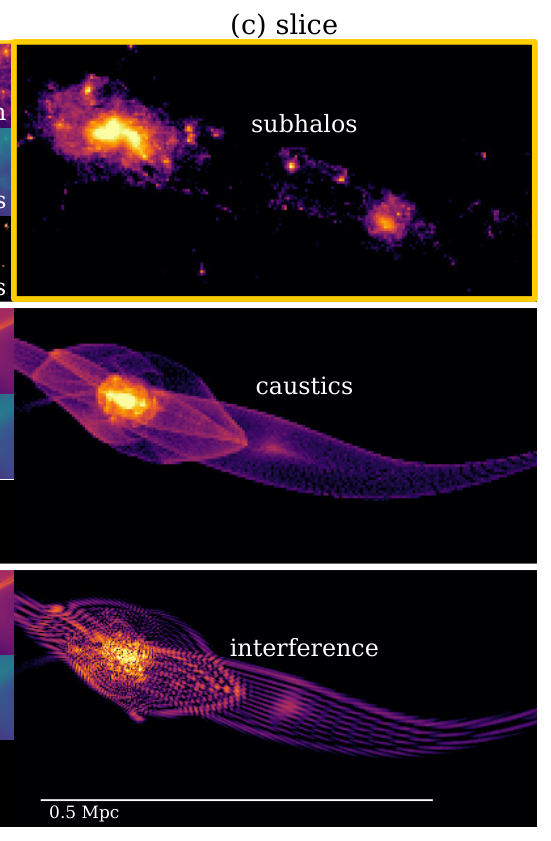
Mocz et al. 2019 — First star-forming structures in fuzzy cosmic filaments arXiv 1910.01653
PhysicsFDM structure formation in filaments
ApproachClassical spectral Schrödinger–Poisson
ResultSolitons, caustics & interference along filaments; first-star formation delayed
Mocz fuzzy filaments
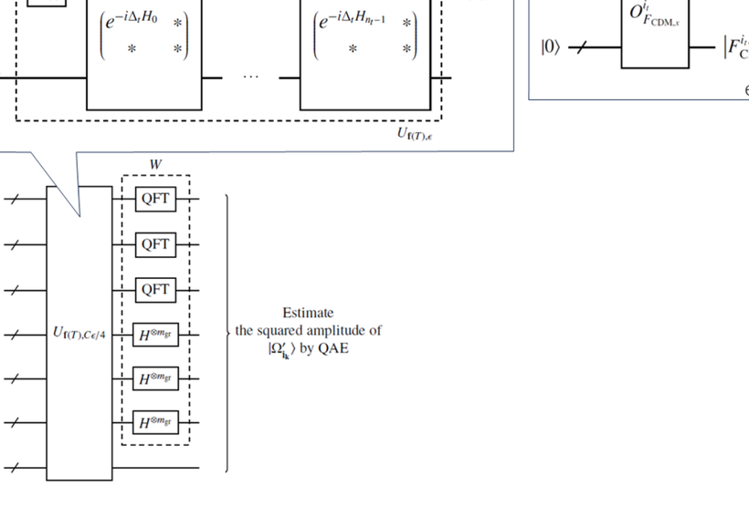
Miyamoto et al. 2024 — Quantum algorithm for the Vlasov simulation of LSS with massive neutrinos ✓ reproduced · this deck arXiv 2310.01832 · PRR 6, 013200
PhysicsMassive-neutrino hot dark matter / large-scale structure
ApproachQuantum algorithm, Vlasov→Schrödinger (digital)
ResultÕ(ngr+nt) vs classical O(ngr⁶); one CDM force mode drives one density mode
Miyamoto quantum Vlasov circuit
Neutral-atom & optical-lattice quantum simulators · analog
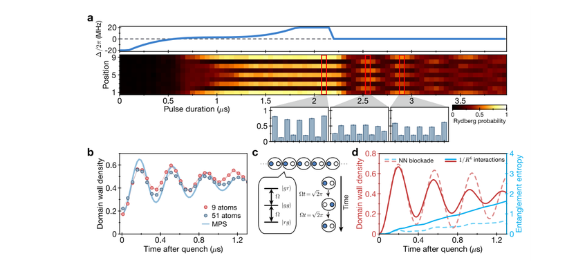
Bernien et al. 2017 — Probing many-body dynamics on a 51-atom quantum simulator arXiv 1707.04344 · Nature
PhysicsMany-body dynamics / quantum scars
ApproachRydberg atom array, 51 qubits (analog)
ResultZ₂-ordered phases; persistent oscillations (scars) after a rapid quench
Bernien 51-atom dynamics
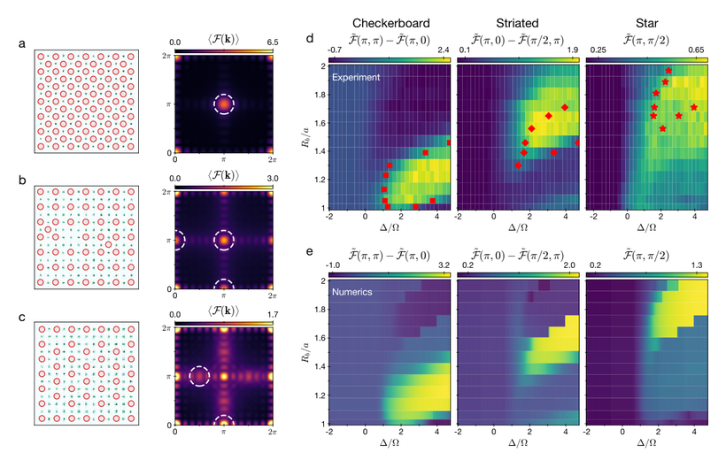
Ebadi et al. 2021 — Quantum phases of matter on a 256-atom programmable quantum simulator arXiv 2012.12281 · Nature
PhysicsQuantum phases of matter & criticality
ApproachRydberg atom array, 256 qubits (analog)
ResultMapped checkerboard / striped / star phases; quantum Kibble–Zurek scaling
Ebadi 256-atom phases
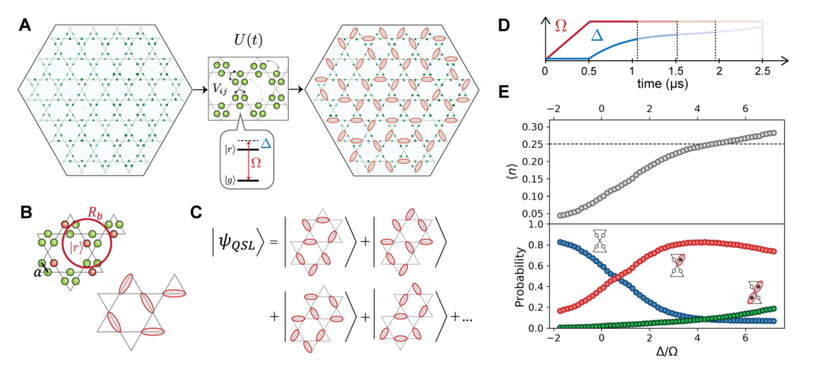
Semeghini et al. 2021 — Probing topological spin liquids on a programmable quantum simulator arXiv 2104.04119 · Science
PhysicsTopological order / quantum spin liquid
ApproachRydberg array on kagome links, 219 atoms (analog)
ResultToric-code-type spin liquid detected via topological string operators
Semeghini spin liquid
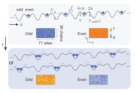
Yang et al. 2020 — Observation of gauge invariance in a 71-site Bose–Hubbard quantum simulator arXiv 2003.08945 · Nature
PhysicsU(1) lattice gauge theory / Gauss's law
ApproachOptical lattice, Bose–Hubbard, 71 sites (analog)
ResultObserved emergent gauge invariance (Gauss's law) in cold atoms
Yang 71-site gauge invariance
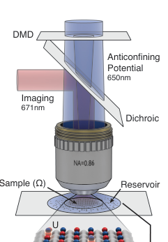
Mazurenko et al. 2017 — A cold-atom Fermi–Hubbard antiferromagnet arXiv 1612.08436 · Nature
PhysicsFermi–Hubbard antiferromagnetism (high-Tc)
ApproachOptical lattice + quantum-gas microscope (analog)
ResultLong-range antiferromagnetic order (staggered magnetization) reached
Mazurenko Fermi-Hubbard microscope
Digital quantum processors · superconducting & trapped-ion
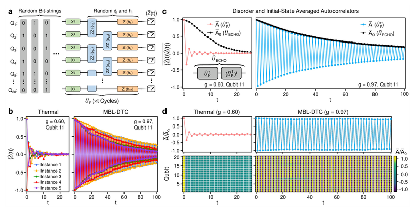
Mi et al. 2021 — Time-crystalline eigenstate order on a quantum processor arXiv 2107.13571 · Nature
PhysicsDiscrete time crystal (non-equilibrium phase)
ApproachSuperconducting qubits (Google Sycamore) (digital)
ResultObserved stable eigenstate-ordered DTC across generic initial states
Mi time crystal
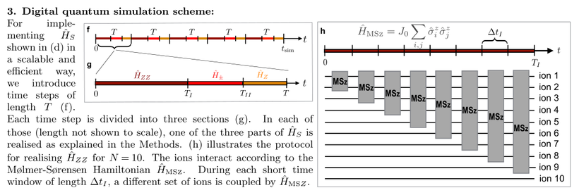
Martinez et al. 2016 — Real-time dynamics of lattice gauge theories with a few-qubit quantum computer arXiv 1605.04570 · Nature
PhysicsLattice gauge theory (Schwinger model) dynamics
ApproachTrapped-ion quantum computer (digital)
ResultFirst digital simulation of Schwinger pair-creation; gauge invariance preserved
Martinez lattice gauge theory
Kokail et al. 2019 — Self-verifying variational quantum simulation of lattice models arXiv 1810.03421 · Nature
PhysicsLattice gauge theory (Schwinger model) ground states
ApproachTrapped-ion variational, 20 qubits (hybrid digital)
ResultVariational ground states + energies/gaps with built-in self-verification
Kokail self-verifying VQS
Quantum computing · chemistry & materials
Kandala et al. 2017 — Hardware-efficient VQE for small molecules & quantum magnets arXiv 1704.05018 · Nature 549, 242
PhysicsMolecular ground-state energies (H2, LiH, BeH2)
ApproachSuperconducting qubits, hardware-efficient VQE (digital)
ResultBeH2 energy on 6 qubits — largest molecule on a QC then; proof-of-principle
Kandala hardware-efficient VQE
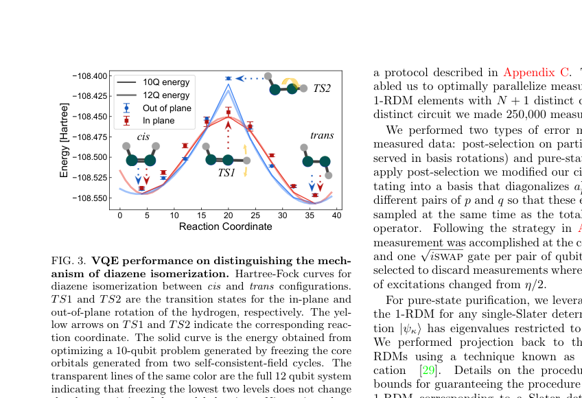
Arute et al. (Google) 2020 — Hartree–Fock on a superconducting qubit quantum computer arXiv 2004.04174 · Science 369, 1084
PhysicsElectronic structure — Hartree–Fock, diazene isomerization
ApproachSuperconducting qubits (Sycamore), up to 12 qubits, VQE (digital)
ResultLargest chemistry VQE at the time; error mitigation → chemically-relevant energies
Arute Hartree-Fock isomerization
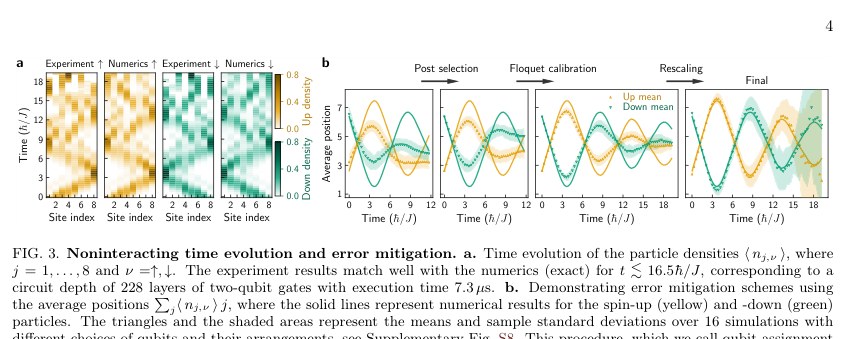
Arute et al. (Google) 2020 — Separated dynamics of charge & spin in the Fermi–Hubbard model arXiv 2010.07965
PhysicsFermi–Hubbard dynamics — spin–charge separation
ApproachSuperconducting qubits (Sycamore), 16 qubits, Trotterized (digital)
ResultCharge & spin spread at different speeds in 1D chains — proof-of-principle
Arute Fermi-Hubbard charge-spin dynamics
Quantum computing · high-energy, nuclear & information
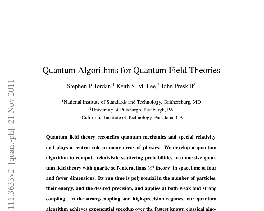
Jordan, Lee & Preskill 2012 — Quantum algorithms for quantum field theories arXiv 1111.3633 · Science 336, 1130
PhysicsRelativistic scattering in φ⁴ scalar QFT
ApproachFault-tolerant quantum algorithm (FT · theory)
ResultPolynomial-time scattering amplitudes, exponential speedup at strong coupling — foundational, not yet run
Jordan-Lee-Preskill quantum algorithms for QFT
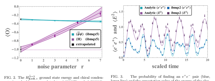
Klco et al. 2018 — Quantum-classical computation of Schwinger-model dynamics arXiv 1803.03326 · PRA 98, 032331
Physics1+1D QED (Schwinger model), real-time dynamics
ApproachIBM superconducting qubits, hybrid variational (digital)
Resulte⁺e⁻ pair production & vacuum persistence on 2 qubits — small demo w/ error mitigation
Klco Schwinger model dynamics
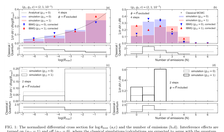
Bauer, de Jong, Nachman & Provasoli 2019 — A quantum algorithm for high-energy-physics simulations arXiv 1904.03196 · PRL 126, 062001
PhysicsCollider parton showers with quantum interference
ApproachQuantum circuit / algorithm, IBMQ demo (digital)
ResultCaptures interfering emission histories classical Markov showers miss — toy-model demo
Bauer parton shower cross sections
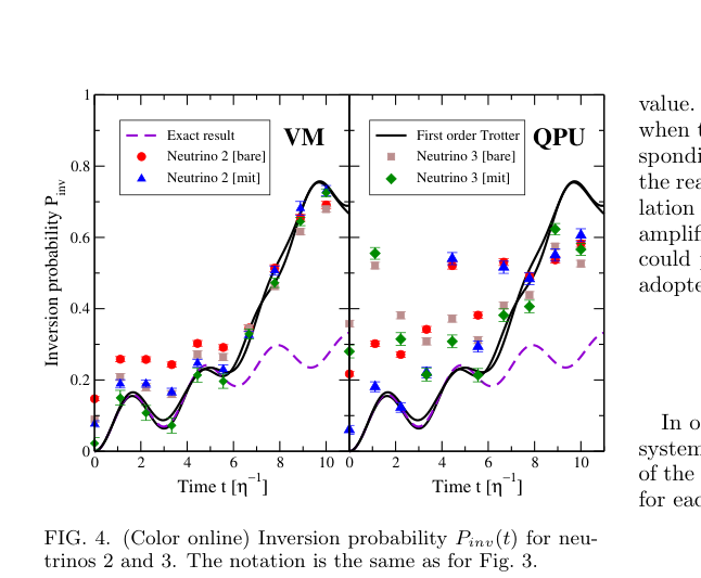
Hall, Roggero, Baroni & Carlson 2021 — Simulation of collective neutrino oscillations on a quantum computer arXiv 2102.12556 · PRD 104, 063009
PhysicsCollective (many-body) neutrino flavor oscillations
ApproachSuperconducting qubits (IBM / Rigetti) (digital)
ResultTracked inversion probability for 2–4 neutrinos; error mitigation needed — proof-of-principle
Hall collective neutrino oscillations
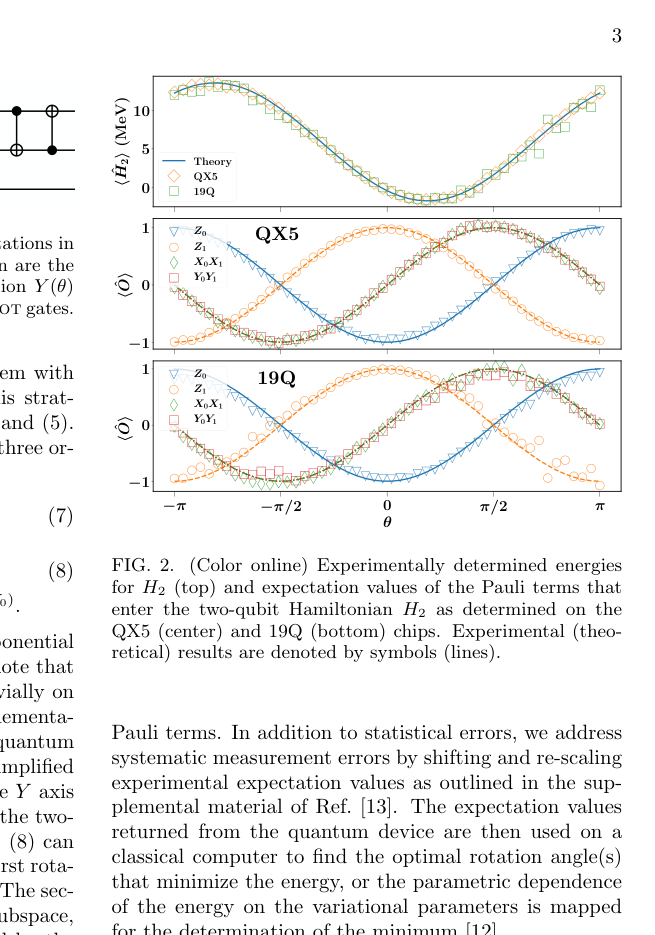
Dumitrescu et al. 2018 — Cloud quantum computing of an atomic nucleus arXiv 1801.03897 · PRL 120, 210501
PhysicsDeuteron binding energy (nuclear structure)
ApproachIBM QX5 & Rigetti 19Q, cloud VQE, 2–3 qubits (digital)
ResultDeuteron ground-state energy via pionless EFT — first atomic nucleus on a QC
Dumitrescu deuteron on quantum chips
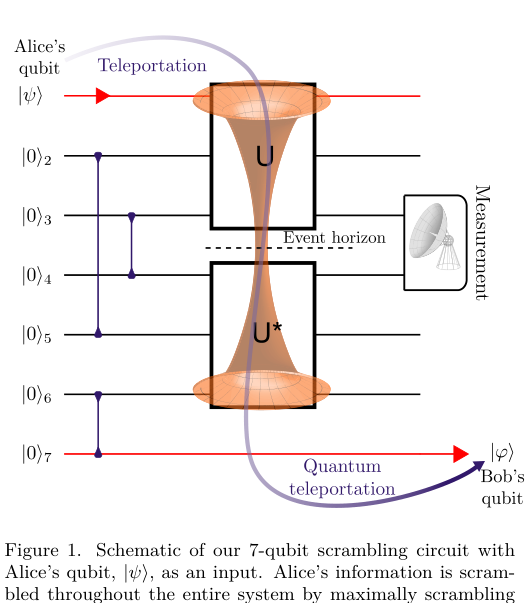
Landsman et al. 2019 — Verified quantum information scrambling arXiv 1806.02807 · Nature 567, 61
PhysicsQuantum information scrambling / black-hole teleportation
ApproachTrapped-ion 7-qubit processor (digital)
ResultTeleportation-fidelity witness verifies scrambling; wormhole-inspired protocol — small-scale demo
Landsman scrambling wormhole circuit
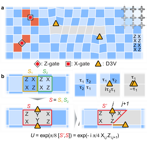
Andersen et al. (Google) 2023 — Non-Abelian braiding of graph vertices in a superconducting processor arXiv 2210.10255 · Nature 618, 264
PhysicsNon-Abelian topological order & anyon braiding
ApproachSuperconducting qubits (Sycamore-class) (digital)
ResultCreated & braided non-Abelian anyons; braids change the measured state — step toward topological QC
Andersen non-Abelian braiding
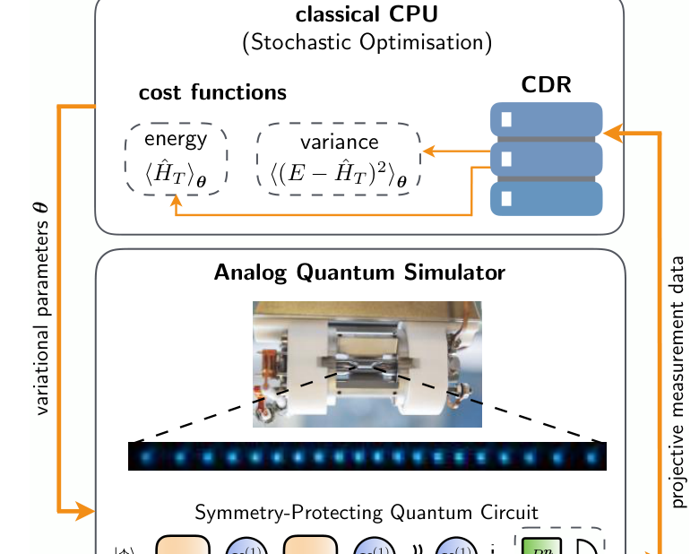
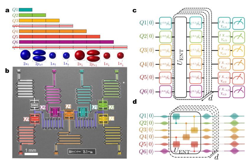
Cosmology in the lab FDM / neutrino cosmology Neutral-atom / lattice Digital QPU QC · chemistry & materials QC · HEP / nuclear / info ✓ our reproductions (VACUA · QVLASOV)
1 / 12